Predicting Drone Signal Drops: A Mathematical Breakthrough

TL;DR: Drone signal drops are a major headache, often unpredictable because the continuous physical signal strength doesn't directly translate to the "good or bad" states our communication systems see. This new research offers a direct mathematical formula to bridge that gap. It maps physical signal fading to a simple "good/bad" channel model, allowing engineers to accurately predict how long a signal will stay reliable based on its "smoothness" and correlation. This means faster, more confident drone designs with smarter communication protocols, leading to far more resilient autonomous flights.

Decoding the Invisible: Why Your Drone's Signal Drops

Ever wonder why your drone's signal sometimes drops out for no apparent reason, or why some flight paths seem more prone to connection hiccups? It's not always interference you can see. Invisible forces, like signal fading, constantly battle your drone's radio link. This new research provides a direct mathematical bridge between how your drone's signal strength fluctuates in the air and how those fluctuations translate into actual communication reliability at the software level. It's about demystifying the invisible and giving engineers the tools to build more resilient drone communication systems.

The Simulation Trap: Why Current Approaches Fall Short

Currently, engineers design drone communication systems by modeling signal strength at a physical level – thinking about dB drops and statistical distributions like correlated Gaussian processes. But software and link-layer protocols, like those handling error correction or retransmissions, operate on a simpler "good or bad" channel state. Bridging these two views has always been a pain point.

You either run massive, time-consuming simulations to see how physical fading affects link-layer performance, or you rely on continuous-time approximations that don't quite give you the discrete, slot-by-slot probabilities you need for real-world digital communication. This guesswork means over-engineering systems (adding unnecessary weight, power, and cost) or, worse, under-engineering them and risking critical link failures mid-flight. Until now, a direct, exact method to connect the "how much signal" to the "is it working?" has been elusive.

The Mathematical Bridge: From Wavy Lines to Good/Bad States

The core innovation here is a closed-form mathematical solution that directly maps a physical-layer Gaussian fading model to a link-layer Gilbert-Elliott (GE) two-state Markov chain. Think of it this way: the physical layer sees a continuous, fluctuating signal (like a wavy line on an oscilloscope). The link layer sees discrete time slots, each either "good" (decodable) or "bad" (not decodable). The paper introduces a threshold: if the signal strength at a given slot is above this threshold, it's a "good" state; below it, it's "bad."

The trick is using Owen's T-function, a specialized integral, to calculate the transition probabilities (p01 and p10) of the GE model. These probabilities tell you how likely the channel is to switch from good to bad, or bad to good, in the next time slot. Crucially, these formulas only depend on the one-step correlation coefficient (ρ) of the underlying Gaussian fading process. This ρ essentially captures how "sticky" the fading is – does a bad signal stay bad, or does it bounce around quickly?

The paper also highlights a critical distinction: the "smoothness" of the underlying fading process matters.

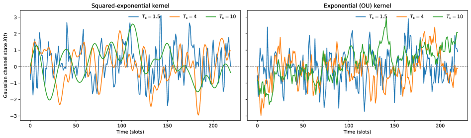Figure 2: Sample paths of the stationary Gaussian fading process for three values of Tc. Left: squared-exponential kernel (1) (smooth paths). Right: exponential kernel (2) (rougher paths due to the non-differentiable covariance at the origin). Both panels use the same Tc values and random seed to highlight the smoothness difference.

As seen in Figure 2, a "smooth" kernel (like squared-exponential) creates more gradual signal changes, while a "rough" kernel (like exponential/Ornstein–Uhlenbeck) leads to choppier, more abrupt shifts. This difference fundamentally changes how long a channel state persists, as we'll see in the results.

Quantifying Reliability: What the Numbers Tell Us

The paper's key achievement is providing exact, closed-form equations for the GE transition probabilities. For instance, when the threshold equals the mean signal, the formula simplifies to an elementary arcsine identity. This isn't just theoretical; Monte Carlo simulations consistently validate these predictions.

Here's what they found:

• Persistence Time: The expected duration a channel stays in a "good" or "bad" state (E[T_GE]) behaves differently based on the fading kernel:
  • For smooth (squared-exponential) kernels, persistence time grows linearly with the correlation length (T_c).
  • For rough (exponential) kernels, persistence time grows only as the square root of T_c. This is a significant difference that impacts how you design robust communication.

Figure 4: Expected persistence time E[T_GE] versus Tc for S/σ=0. Left: squared-exponential kernel with exact theory (16) (solid), linear asymptote (33) (dashed), and Monte Carlo (circles). Right: exponential kernel with exact theory (solid), Tc square root asymptote (34) (dashed), and Monte Carlo (circles). The contrasting growth rates (linear vs. Tc square root) are clearly visible.

Figure 4 clearly illustrates this divergence in growth rates, with the theoretical curves (solid lines) perfectly matching Monte Carlo simulations.

• Threshold Impact: The chosen signal strength threshold S/σ significantly affects persistence, as shown in Figure 5. This means engineers can tune their "good/bad" definition to better match their application's needs.

Figure 5: Effect of the threshold level on E[T_GE], both kernels. Left: squared-exponential. Right: exponential. Solid lines are the closed-form theory (16); markers show Monte Carlo means with 95% CIs. Only nonnegative thresholds are shown (the mapping is symmetric under S/σ↦−S/σ). The square-root scaling of the exponential kernel is evident in the sublinear curvature of the right panel.

• Markovian Approximation: The paper also quantifies when a simple first-order GE chain is "good enough" and when more complex models are needed.
  • They use two diagnostics: the "one-step Markov gap" (local accuracy) and "run-length total-variation distance" (global path fidelity).
  • Intriguingly, these two diagnostics can trend in opposite directions, as seen in Figure 1, revealing the nuances of local versus global channel behavior.

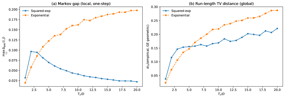Figure 1: Two diagnostics for the matched first-order GE chain (S/σ=0, both kernels). (a) Maximum Markov gap: a local, one-step measure that decreases for the squared-exponential kernel but increases for the exponential kernel. (b) Run-length TV distance: a global, path-shape measure that increases with Tc/D for both kernels. The opposing trends in the squared-exponential case reflect the distinction between local conditional accuracy and global run-length fidelity.

For instance, Figure 7 shows that for an exponential kernel, a second-order Markov correction is far more effective in reducing the total-variation distance, suggesting that a simple first-order GE might not always capture the full picture for rougher fading.

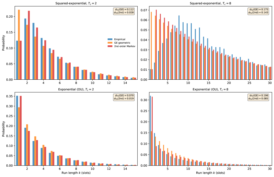Figure 7: Run-length distributions for state-1 runs (S/σ=0). Top row: squared-exponential kernel. Bottom row: exponential kernel. Left column: Tc=2. Right column: Tc=8. Each panel annotates the total-variation distances dTV for the first-order GE geometric and second-order Markov fits. At Tc=2 the exponential kernel already shows a better GE fit than the squared-exponential (0.070 vs. 0.112). At Tc=8 both kernels develop heavier-than-geometric tails, but the second-order Markov correction is far more effective for the exponential kernel (dTV drops from 0.196 to 0.085) than for the squared-exponential (0.175 to 0.143), reflecting the shallower binary non-Markovity of the exponential kernel.

Smarter Skies: What This Means for Drones

This research is a big deal for anyone designing or operating drones where reliable communication is paramount.

• Predictive Power: Engineers can now accurately predict channel reliability without resource-intensive simulations. This means faster design cycles and more confident deployment.
• Smarter Communication Protocols: Knowing the exact transition probabilities for good/bad channel states allows for the design of highly optimized error correction codes, adaptive data rates, and intelligent retransmission strategies. If you know the channel is likely to stay bad for X milliseconds, you can adapt your protocol to handle that.
• Robust Autonomous Missions: For autonomous drones, understanding communication link dynamics is crucial. This model helps predict when a drone might temporarily lose reliable command and control or telemetry. This information can be fed into flight controllers to trigger pre-programmed behaviors, like hovering or returning home, before a full loss of link occurs.
• FPV and Data Links: For FPV racers, clear video feeds are everything. For industrial drones collecting data, robust data links are non-negotiable. This work helps build systems that can better anticipate and manage signal degradation. It’s about building systems that don't just react to failure, but anticipate it.

The Road Ahead: Limitations and Unanswered Questions

While powerful, this bridge isn't a silver bullet.

• Stationary Assumption: The model assumes the underlying Gaussian fading process is stationary. In reality, a drone's environment and movement can cause non-stationary fading, where statistical properties change over time (e.g., flying from open field to urban canyon). Adapting this model to non-stationary scenarios would be a critical next step.
• Parameter Estimation: While the formulas are closed-form, applying them requires accurate real-world estimates of the Gaussian fading process's parameters, like its mean, variance, and, crucially, the one-step correlation coefficient (ρ) and correlation length (T_c). Obtaining these reliably in dynamic drone environments can be challenging.
• Focus on First-Order: The paper primarily focuses on the first-order Gilbert-Elliott model, though it does discuss its limitations and the need for higher-order Markov chains (as seen in Figure 7). For highly dynamic or complex fading environments, a simple two-state, first-order model might not fully capture the channel's memory.
• Mitigation, Not Solution: This research provides a powerful modeling tool to understand channel behavior, but it doesn't directly offer solutions for mitigating bad channel states. That's still up to the system designer, albeit with much better information.

Getting Your Hands Dirty (Theoretically)

Directly applying Owen's T-function and the associated mathematics to raw signal data isn't a typical weekend project for most hobbyists without a strong signal processing background. However, the insights from this paper are highly relevant. If you're building drone communication systems, even at a high level, understanding the difference between "smooth" and "rough" fading environments, and how that impacts expected signal persistence, can inform your component choices and protocol designs. For those with programming skills, libraries for numerical integration and statistical analysis (like SciPy in Python) could be used to implement these formulas if you have access to raw signal strength data from your drone's radio. There's no specific open-source hardware mentioned, but the principles apply to any digital radio link.

This work on communication reliability also intersects with other critical areas of drone autonomy. For instance, the paper on "SFFNet: Synergistic Feature Fusion Network With Dual-Domain Edge Enhancement for UAV Image Object Detection" by Zhang et al. reminds us that while robust communication is vital, a drone also needs to interpret its surroundings accurately. If your drone's signal is intermittent, its ability to reliably detect objects, even with noisy backgrounds, becomes even more critical for safe autonomous flight.

Similarly, if a drone's communication is compromised, its internal reasoning capabilities become paramount. The work by Zhang et al. on "Understanding the Role of Hallucination in Reinforcement Post-Training of Multimodal Reasoning Models" explores how AI models can "hallucinate" or misinterpret data. For a drone, this means its AI needs to reason accurately even when commands or sensory data might be delayed or incomplete due to comms issues, preventing dangerous misjudgments. Finally, "CoME-VL: Scaling Complementary Multi-Encoder Vision-Language Learning" by Deria et al. on advanced Vision-Language Models (VLMs) offers another angle: better VLMs could help drones understand complex, sparse commands from human operators or interpret environmental cues more intelligently, especially when a perfectly stable, high-bandwidth communication link isn't guaranteed. All these papers underscore the need for resilience and intelligence when the invisible forces of signal disruption strike.

Beyond Guesswork: The Future of Drone Comms

Ultimately, this work moves us closer to a future where drone communication isn't just reliable by brute force, but intelligently resilient, built on a foundation of deep mathematical understanding rather than mere guesswork.

---

Paper Details

Title: From Gaussian Fading to Gilbert-Elliott: Bridging Physical and Link-Layer Channel Models in Closed Form Authors: Bhaskar Krishnamachari, Victor Gutierrez Published: April 2026 arXiv: 2604.03160 | PDF